# libraries
library(bayesrules)
library(dplyr)
library(tidyr)
library(gt)
library(tibble)
library(ggplot2)
data(fake_news)
fake_news <- tibble::as_tibble(fake_news)Chapter 2 Notes
Note: these notes are a work in progress
In this chapter we step through an example of “fake” vs “real” news to build a framework to determine the probability of real vs fake of a new news article titled “The President has a secret!”
We then go on to build a probability known as the Binomial model using the Bayesian framework
What is the proportion of news articles that were labeled fake vs real.
fake_news |> head()# A tibble: 6 × 30
title text url authors type title…¹ text_…² title…³ text_…⁴ title…⁵
<chr> <chr> <chr> <chr> <fct> <int> <int> <int> <int> <int>
1 Clinton's E… "0 S… http… <NA> fake 17 219 110 1444 0
2 Donald Trum… "\n\… http… <NA> real 18 509 95 3016 0
3 Michelle Ob… "Mic… http… Sierra… fake 16 494 96 2881 1
4 Trump hits … "“Cr… http… Jack S… real 11 268 60 1674 0
5 Australia V… "Whe… http… Blair … fake 9 479 54 2813 0
6 It’s “Trump… "Lik… http… View A… real 12 220 66 1351 1
# … with 20 more variables: text_caps <int>, title_caps_percent <dbl>,
# text_caps_percent <dbl>, title_excl <int>, text_excl <int>,
# title_excl_percent <dbl>, text_excl_percent <dbl>, title_has_excl <lgl>,
# anger <dbl>, anticipation <dbl>, disgust <dbl>, fear <dbl>, joy <dbl>,
# sadness <dbl>, surprise <dbl>, trust <dbl>, negative <dbl>, positive <dbl>,
# text_syllables <int>, text_syllables_per_word <dbl>, and abbreviated
# variable names ¹title_words, ²text_words, ³title_char, ⁴text_char, …fake_news |>
group_by(type) |>
summarise(
total = n(),
prop = total / nrow(fake_news)
) # A tibble: 2 × 3
type total prop
<fct> <int> <dbl>
1 fake 60 0.4
2 real 90 0.6If we let \(B\) be the event that a news article is “fake” news, and \(B^c\) be the event that a news article is “real”, we can write the following:
\[P(B) = .4\] \[P(B^c) = .6\]
This is the first “clue” or set of data that we have to build into our framework. Namely, majority of articles are “real”, therefore we could simply predict that the new article is “real”. This updated sense or reality now becomes our priors.
Getting additional data, and updating our priors, based on additional data. The new observation we make is the use of exclamation marks “!”. We note that the use of “!” is more frequent in news articles labeled as “fake”. We will want to incorporate this into our framework to decide whether the new incoming should be labelled as real or fake.
Likelihood
So in our case, we don’t know whether this new incoming article is real or not, but we do know that the title has an exclamation mark. This means we can evaluate how likely this article is real or not given that it contains an “!” in the title using likelihood functions. We can formualte this as:
\[L(B|A) \text{ vs } L(B^c|A)\]
And perform the computation in R as follows:
# if fake, what are the proprotions of ! vs no-!
prop_of_excl_within_type <- fake_news |>
    group_by(type, title_has_excl) |>
    summarise(
        total = n()
    ) |>
    ungroup() |>
    group_by(type) |>
    summarise(
        has_excl = title_has_excl,
        prop_within_type = total / sum(total)
    )
prop_of_excl_within_type |>
pivot_wider(names_from = "type", values_from = prop_within_type) |>
gt() |>
gt::cols_label(
has_excl = "Contains Exclamtion",
fake = "Fake",
real = "Real") |>
gt::fmt_number(columns=c("fake", "real"), decimals = 3) |>
gt::cols_width(everything() ~ px(100))| Contains Exclamtion | Fake | Real |
|---|---|---|
| FALSE | 0.733 | 0.978 |
| TRUE | 0.267 | 0.022 |
The table above also shows the likelihoods for the case when an article does not contain exclamation point in the title as well. It’s really important to note that these are likelihoods, and its not the case that \(L(B|A) + L(B^c|A) = 1\) as a matter of fact this value evaluates to a number less than one. However, since we have that \(L(B|A) = .267\) and \(L(B^c|A) = .022\) then we have gained additional knowledge in knowing the use of “!” in a title is more compatible with a fake news article than a real one.
Up to this point we can summarize our framework as follows
| event | \(B\) | \(B^c\) | Total |
|---|---|---|---|
| prior | .4 | .6 | 1 |
| likelihood | .267 | .022 | .289 |
Our next goal is come up with normalizing factors in order to build our probability table:
| \(B\) | \(B^c\) | Total | |
|---|---|---|---|
| \(A\) | (1) | (2) | |
| \(A^c\) | (3) | (4) | |
| Total | .4 | .6 | 1 |
A couple things to note about our table (1) + (3) = .4 and (2) + (4) = .6. (1) + (2) + (3) + (4) = 1.
(1.) \(P(A \cap B) = P(A|B)P(B)\) we know the likelihood of \(L(B|A) = P(A|B)\) and we also know the prior so we insert these to get \[ P(A \cap B) = P(A|B)P(B) = .267 \times .4 = .1068\]
(3.) \(P(A^c \cap B) = P(A^c|B)P(B)\) in this case we do know the prior \(P(B) = .4\), but we don’t directly know the value of \(P(A^c|B)\), however, we note that \(P(A|B) + P(A^c|B) = 1\), therefore we compute \(P(A^c|B) = 1 - P(A|B) = 1 - .267 = .733\) \[ P(A^c \cap B) = P(A^c|B)P(B) = .733 \times .4 = .2932\]
we now can confirm that \(.1068 + .2932 = .4\)
Moving on to (2), (4)
(2.) \(P(A \cap B^c) = P(A|B^c)P(B^c)\). In this case know the likelihood \(L(B^c|A) = P(A|B^c)\) and we know the prior \(P(B^c)\) therefore, \[P(A \cap B^c) = P(A|B^c)P(B^c) = .022 \times .6 = .0132\]
(4.) \(P(A^c \cap B^c) = P(A^c|B^c)P(B^c) = (1 - .022) \times .6 = .5868\)
and can confirm that \(.0132 + .5868 = .6\)
and we can fill the rest of the table:
| \(B\) | \(B^c\) | Total | |
|---|---|---|---|
| \(A\) | .1068 | .0132 | .12 |
| \(A^c\) | .2932 | .5868 | .88 |
| Total | .4 | .6 | 1 |
An important concept we implemented in above is the idea of total probability
In the above calculations we also step through joint probabilities
At this point we are able to answer the question, “What is the probability, the new article is fake?”. Given that the new article has an exclamation point, we can zoom into the top row of the table of probabilitties. Within this row we have probabilities \(.1068/.12 = .833\) for fake and \(.0132 / .12 = .11\) for real.
This is essentially Baye’s Rule. We developed a posterior probability for an event \(B\) given some observation \(A\). We did so by combining the likelihood of event \(B\) given some new data \(A\) and the prior probability of event \(B\). More formally we have the following definition:
Simualation
articles <- tibble::tibble(type = c("real", "fake"))

priors <- c(.6, .4)

articles_sim <- sample_n(articles, 10000, replace = TRUE, weight = priors)
articles_sim |>
ggplot(aes(x = type)) + geom_bar()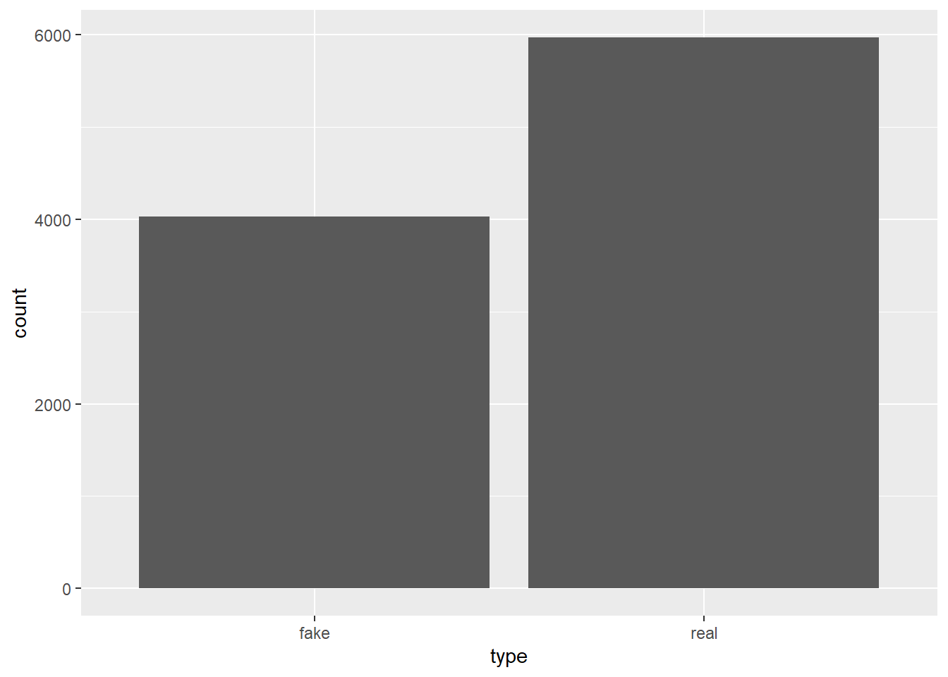
and a summary table
articles_sim |>
    group_by(type) |>
    summarise(
        total = n(),
        prop = total / nrow(articles_sim)
    ) |>
    gt()|>
gt::cols_width(everything() ~ px(100))| type | total | prop |
|---|---|---|
| fake | 4031 | 0.4031 |
| real | 5969 | 0.5969 |
the simulation of 10,000 articles shows us very nearly the same priors we had from the data. We can now add the exclamation usage into the data.
articles_sim <- articles_sim |>
    mutate(model_data = case_when(
        type == "fake" ~ .267,
        type == "real" ~ .022
    ))
The plan here is to iterate through the 10,000 samples and use the data_model value to assign either, “yes” or “no” using the sample function.
data <- c("yes", "no")

articles_sim <- articles_sim |>
    mutate(id = row_number()) |>
    group_by(id) |>
    mutate(usage = sample(data, 1, prob = c(model_data, 1 - model_data)))
articles_sim |>
group_by(usage, type) |>
summarise(
total = n()
) |>
pivot_wider(names_from = type, values_from = total)# A tibble: 2 × 3
# Groups: usage [2]
usage fake real
<chr> <int> <int>
1 no 2955 5845
2 yes 1076 124articles_sim |>
ggplot(aes(x = type, fill = usage)) +
geom_bar() +
scale_fill_discrete(type = c("gray8", "dodgerblue4"))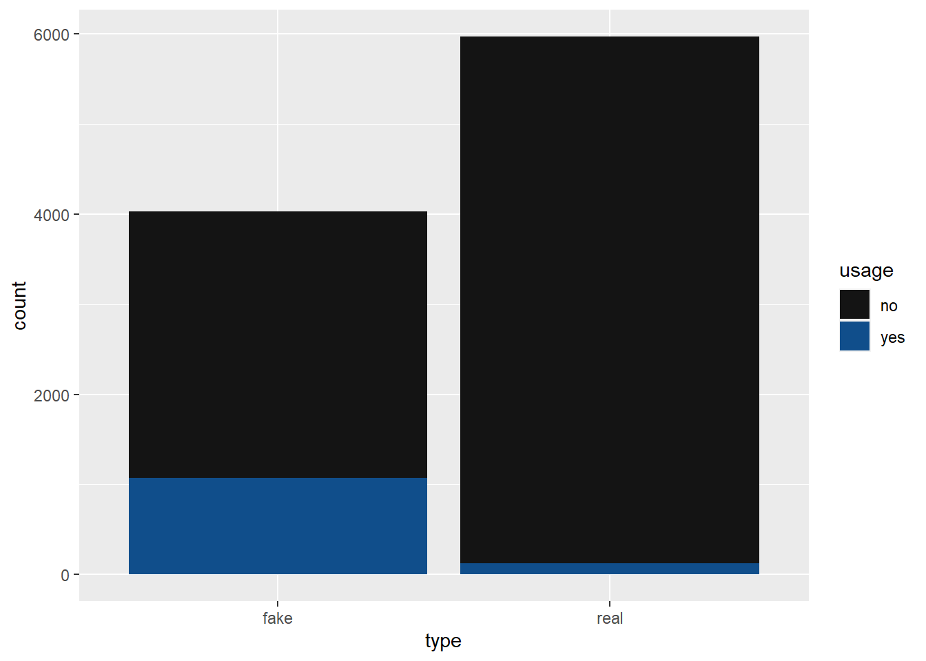
So far have compute both the priors and likelihoods, we can simply filter our data to reflect the incoming article and determine our posterior.
articles_sim |>
    filter(usage == "yes") |>
    group_by(type) |>
    summarise(
        total = n()
    ) |>
    mutate(
        prop = total / sum(total)
    )
# A tibble: 2 × 3
type total prop
<chr> <int> <dbl>
1 fake 1076 0.897
2 real 124 0.103Binomial Model and the chess example
The example used here is the case of a chess match between a human and a computer “Deep Blue”. The set up is such that we know the two faced each other in 1996, in which the human won. There is a rematch scheduled for the next 1997. We would like to model the number of games out of 6 that the human can win.
Let \(\pi\) be the probability that the human wins any one match against the computer. To simplify things greatly we assume that \(\pi\) takes on values of .2, .5, .8. We also assume the following prior (we are told in the book that we will learn how to build these later on):
| \(\pi\) | .2 | .5 | .8 | total |
|---|---|---|---|---|
| \(f(\pi)\) | .10 | .25 | .65 | 1 |